Xie C, Wang J, Zhang Z, et al. Adversarial examples for semantic segmentation and object detection[C]//Proceedings of the IEEE International Conference on Computer Vision. 2017: 1369-1378.
1. Overview
In this paper, it proposed Dense Adversary Generation (DAG)
- optimize a loss function over a set of pixels/proposals for generating adversarial perturbations
- consider all targets simultaneously and optimizes the overall loss function
- 150~200 iteration
- change IOU to preserve more proposals. generating adversarial example is more difficult in detection then segmentation (O(N*N) vs O(N), N pixels)
- add two or more heterogeneous perturbations significantly increase the transferability
1.1. Related Work
- FGSM
- universal adversarial perturbation
- trained a network to generate adversarial examples for a target model
- ensemble-based approaches to generate adversarial examples with stronger transferability
- forveation-based mechanism to alleviate adversarial examples
- defensive distillation
- train network on adversarial examples
- ensemble adversarial training methods
2. Methods
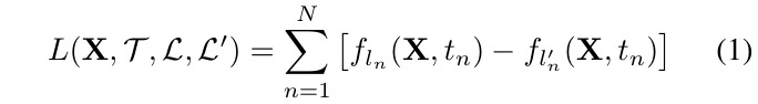
- t_n. n-th target in the image
- X. image
- f_{l}. the score of l class
- l_n. the class of target t_n
- l_n’. the any class except the gt class l_n

- T. activate target set (predict right)

- normalize r

- γ = 0.5

- r. sum of all r_m
- X^. the mean image of X. often X-X^
3. Details
- target set selection is more difficult in detection task.
when the adversarial perturbation r is added t the original image X, a different set of proposals may be generated according to the net input X+r. - incrase the threshhold of NMS in RPN(IOU: 0.7 to 0.9 → 300 proposals to 3000 proposals)
4. Experiments
4.1. Comparison

- permuted perturbations cause negligible accuracy drop
- indicate that it is the spatial structure of r, instead of its magnitude, contributes in generating adversarial examples
4.2. Control Output

4.3. Denseness of Proposals

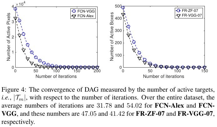
4.4. Convergence
4.5. Perceptibility

- K. number of pixels
- segmentation. 2.6e-3, 2.5e-3, 2.9e-3, 3e-3 on FCN-Alex, FCN-Alex, FCN-VGG, FCN-VGG
- detection. 2.4e-3, 2.7e-3, 1.5e-3, 1.7e-3
4.6. Transferability
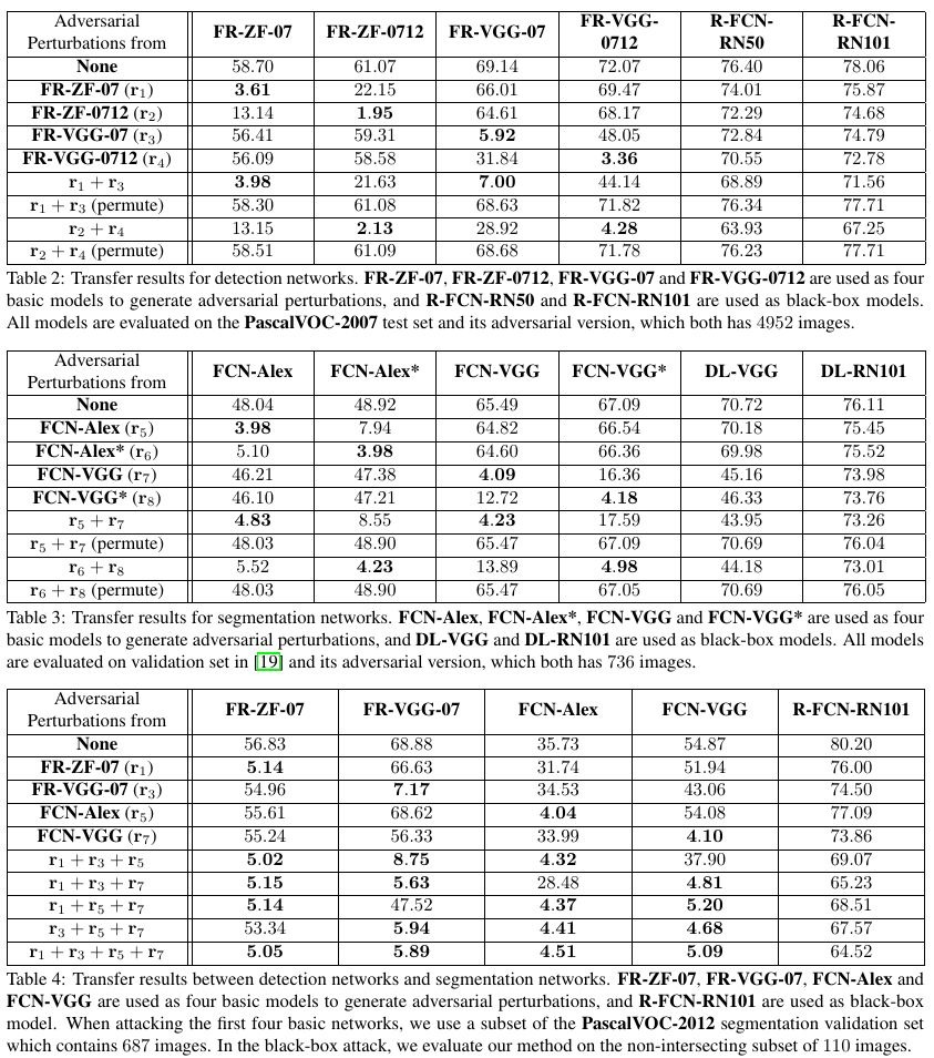
4.6.1. Cross-Training Transfer
- perturbation learn from one network to another network with same architecture but different dataset
4.6.2. Cross-Network Transfer
- through different network structures
4.6.3. Cross-Task Transfer
- perturbation generated from one task to attack another task
- drop significantly between same network (FCN-VGG, FR-VGG-07)
4.6.4. Combining Heterogeneous Perturbations
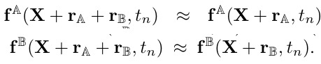
- add multiple adversarial perturbation often works better than adding a single source of perturbation